Exploratory Data Analysis
You can download a copy of the code described in this page as an ipython notebook or a pdf
We extracted data for 20 variables which built the basis for the Exploratory Data Analysis. All together we had 9974 observations.
These are the variables we used for our analysis:
- won: Response variable. 1 if the candidate won, 0 otherwise
- district: Congressional districts name
- is_incumbent: Whether an incumbent is running for re-election
- name: The candidate’s name
- party: The candidate’s party
- percent: The percentage of votes received by the candidate
- state: The name of the state
- votes: The number of votes received by the candidate
- year: The year of the election.
- first_time_elected: The year of the first election won in this district by the candidate (NaN if not applicable).
- count_victories: The number of elections won in this district by the candidate
- unemployement_rate: The unemployment rate of the district (or of the country if the information was not available) for the month before the election.
- is_presidential_year: 1 if there is a presidential election this year, 0 otherwise.
- president_can_be_re_elected: Can the president stand for re-election ? 1 = Yes, 0 = No
- president_party: The president’s party (R or D)
- president_overall_avg_job_approval: The presidential job approval ratings (available from Truman - to Trump). Source: Gallup.
- last_D_house_seats: The number of house seats won by democrats at the last elections
- last_R_house_seats: The number of house seats won by republicans at the last elections
- last_house_majority: Which party have the majority (R or D)
- fundraising: How much money does the candidate raised for the campaign
Our data for the training set will be all data excluding the year 2018. The test set will be restricted to the year 2018 only. Both datasets are very good balanced regarding the values in the response variable:

So we don’t need to resample data, stratify or generate any synthetic samples.
Data imputation
The first data quality corrections were already done when extracting the data from the different sources. Sometimes we faced the situation that the data quality was bad and we even had to add data manually. With the final preparation of the data we had to deal with the remaining missing values. The solution for most of the missing values was to group the data for state, district and/or year and take the mean. This is the result of the data imputation process. This table shows where we had missing values and how we corrected them:
| Variable | # NaN | Data imputation | # NaN after imputation |
|---|---|---|---|
| district | 0 | 0 | |
| is_incumbent | 112 | if grouped sum for state/district/year > 0 then assign 0, else 1 | 0 |
| name | 0 | 0 | |
| party | 0 | 0 | |
| percent | 15 | calculated with mean of votes from state district and year | 0 |
| state | 0 | ||
| votes | 58 | replace with mean of votes from state and district | 0 |
| won (response variable) | 0 | 0 | |
| year | 0 | 0 | |
| first_time_elected | 4445 | take value from year if won=1 else 0 | 0 |
| count_victories | 0 | 0 | |
| unemployement_rate | 979 | replace with mean from state and district | 0 |
| is_presidential_year | 102 | Set to 0 | 0 |
| president_can_be_re_elected | 102 | Set to 0 | 0 |
| president_party | 102 | Set to 0 | 0 |
| president_overall_avg_job_approval | 1060 | Version 1: replace with mean from state and district. Version 2: model based imputation |
0 |
| last_D_house_seats | 102 | Replace with mean from state and district | 0 |
| last_R_house_seats | 102 | Replace with mean from state and district | 0 |
| last_house_majority | 102 | Replace with the most common value from state and district | 0 |
| fundraising | 7161 | Version 1: replace with mean from state and district. Version 2: model based imputation |
0 |
The reason for most of these NaN values was because some observations go back to the year 1824 where many information was not yet available. Beside mean imputation we also implemented a function with the possibility for model based imputation. But when testing with the classification models we didn’t see any improvements so we kept the mean imputation method.
Variable selection
We are only using 20 variables in our dataset so a dimension reduction was not that important but for the modeling part we wanted to know about the feature importance.
We used 7 category variables including the response variable. To test if there is a significant relationship between a predictor variable and the response variable we used the Chi-Square test:
The printed result was this:
- Important for the prediction model: president_party (p-value: +0.231, chi2: +2.9)
- Important for the prediction model: state (p-value: +1.000, chi2: +18.5)
- Important for the prediction model: district (p-value: +1.000, chi2: +15.3)
- Important for the prediction model: last_house_majority (p-value: +0.933, chi2: +0.0)
- NOT important for the prediction model: name (p-value: +0.000, chi2: +9938.0)
At the end we could not simply remove the variable “name” from the variable set at this point because it was needed for feature engineering which was done in the modeling part.
To get a sense about the feature importance we used a Random Forest model with one-hot-coding. This method was then also used in the modeling part to decide which variables can be dropped. Variables like state or district for which we had to create dummy variables got a lower feature importance value because they were distributed over several columns.
These are the first 20 variables sorted by importance:
- (0.128, ‘percent’),
- (0.122, ‘votes’),
- (0.092, ‘fundraising’),
- (0.053, ‘unemployement_rate’),
- (0.050, ‘first_time_elected’),
- (0.040, ‘year’),
- (0.031, ‘last_D_house_seats’),
- (0.030, ‘last_R_house_seats’),
- (0.024, ‘count_victories’),
- (0.022, ‘president_overall_avg_job_approval’),
- (0.015, ‘state_California’),
- (0.014, ‘is_incumbent’),
- (0.0128, ‘won’),
- (0.011, ‘district_District 1’),
- (0.011, ‘is_presidential_year’),
- (0.011, ‘district_District 2’),
- (0.009, ‘district_District 4’),
- (0.009, ‘state_Texas’),
- (0.009, ‘district_District 3’),
- (0.008, ‘state_New York’),
Also we used the scatterplot matrix to find out which variables will be important and give us insights about their relevance. During the EDA phase we also experimented already with combining some variables so this is just one of the examples we analyzed. Here we differentiated the observations by the “won” factors:
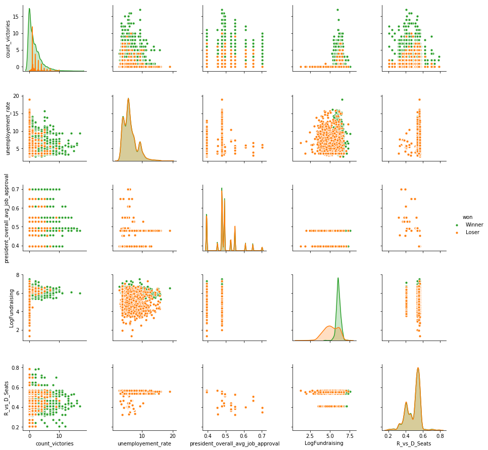
Though we can’t see clear linear correlations or patterns, by differentiating by the winners against the losers, we can see how the green and orange observations are very distinct, in some cases.
Some examples:
- The fund raising of winners is much higher than losers
- Winners reach higher count of victories
Then, we plot only the candidates who won the elections, differentiated by party:
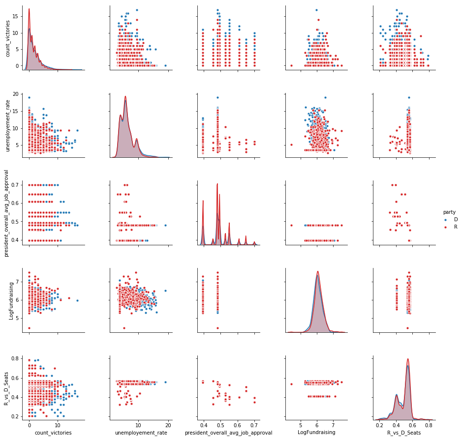
Still we can’t see clear linear correlations or patterns, although we notice that there are some differences:
- Democrats winners reach higher count_victories, sign of a bigger political longevity or district stability
- For a higher unemployment rate, Democrats win more than Republicans
- Democrat winners raise slightly less funds than Republican winners
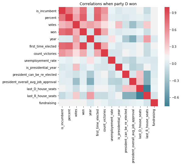
Further we created heat map matrices that give us insights about correlations between the continuous variables. In the plots we differentiated if Democrats or Republicans won. This matrix shows the correlations when the Democrats won together with a colorbar on the right side:
This matrix shows the correlations when the Republicans won:
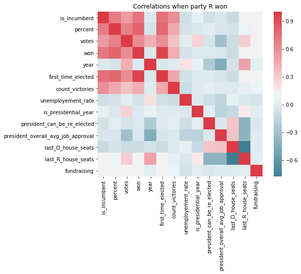
We can see that the strength of the relationships between Democrats and Republicans is very often similar. As expected, the correlations between the variables percent, votes and won will be high.
We also wanted to know about the spread of the data and how the values for Democrats and Republicans compare to each other so we created some boxplots to show this:
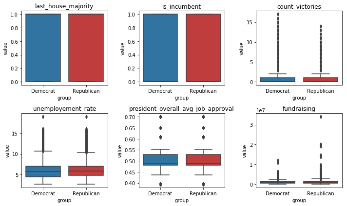
In the modeling phase we will use this information from the EDA phase to be able to create features that improve the model performance and concentrate on the most important features.
Baseline
For the Baseline model we created a very simple data model to check if we have a promising set of features. We used a simple prediction for each district, by just taking the max occurring winner per each district before 2018. Compared to the actual election results in 2018, we get 77% accuracy.
So we are confident to be able to create good models in the modeling phase