Modeling
You can download a copy of the code described in this page as an ipython notebook or a pdf
The main steps we went through for generating our predictions can be split as:
- Feature engineering
- Calculate cross-validation accuracies
- Tuning parameters
- Improving prediction accuracy
- Stacking multiple models
For the modeling part we created a dedicated notebook called “03-Modeling.ipynb”. On this page we will describe our modeling process by referring to functions and other coding elements defined there.
Load data
We start from loading the dataset after data imputation.
Baseline model
We define our baseline model by simply taking the party, per each district, with the highest winning rate.
Here we have defined winnerFilter_ and baselineTrain_. The only difference with the winnerFilter and baselineTrain defined in the 02_EDA.ipynb notebook is that here we refer to parties as 1 and 0, instead than as ‘R’ and ‘D’.
We prepare a dictionary results containing the winner parties of each year, grouped by state and district.
Also, we define districtPredictions and districtAccuracy that merge predictions with actual districts, so that accuracy is calculated on all existing districts, rather than only on the ones for which we have a predicted winner.
In fact:
- based on the training set we might not have a prediction for all districts. As districts are redistributed through the years, one that is in the test set might not exist in the training set, so we have no prediction for it.
- we might have ex aequo winning predictions among candidates of opponent party, which do not lead to a winner prediction.
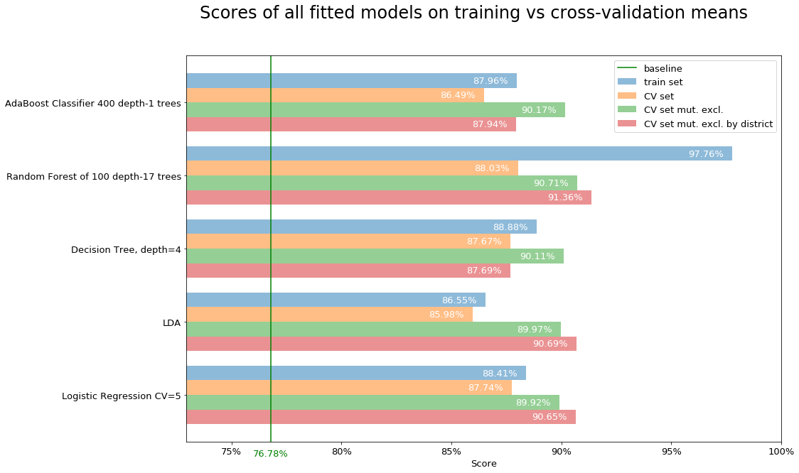
Using the mentioned functions, we calculate the accuracy of the baseline model over the 2018 test set, obtaining a baseline 2018 test accuracy of 76.78%.
This will be the term of comparison for all next models.
Functions definitions
Now we start to define a certain amount of functions, to get the code as modular and clean as possible.
We define a function splitDf for splitting the dataset:
- test set on data belonging to a specified input
year - training set on data from remaining years
- store
state,districtandpartyinformation using the same original index as the main data - drop response features like
percentandvotes, plusstate,districtandname - split into
x_trainandy_train,x_testandy_test, usingwonas response feature - return
x_train,y_train,x_test,y_test,indexed_districtsandindexed_party
Plot functions
Here we define several plotting functions which will be reused through the modeling.
Feature engineering
Our dataset needs to be manipulated quite extensively.
Some examples:
- during the exploration phase we have noticed how the distribution of fundraising is so broad and needs some mathematical transformation.
- We have strings features
- there is a mistake in
first_time_electedfeature, which has values ‘in the future’ compared to the observation year. - We have to predict if a candidate will win, anyway many features are not related to the candidate, rather are absolute data: for example, saying that a district is partisan for the candidate’s party should be more informative than saying that it is partisan for party A or B.
Partisanship
deductPartisanship:
- for a given
x_trainset, we look at the prevalence of one party to win in each district, looking at they_traindata. - a district is partisan for a specific party, if the winning rate of that party in history is greater than 66.7%. (we assign 3=traditionally Republican, 2=traditionally Democrat)
- if no parties have a winning rate grater than 2/3 (66.7%), then that is a “swing district” (we assign 1)
- if we don’t have enough historical data, because the district is new, we don’t conclude anything (we assign 0)
Then with assignPartisanship we assign the 3,2,1 or 0 value for partisanship to each district in the x_test data, using the deductPartisanship function.
This is a model by itself, with a train step and a predict step. When using this feature into another model, we do a kind of stacking, in fact.
Design features, drop features
In the designFeatures function we applied mathematical transformations, convert strings to numbers, produced an amount of interaction terms and fixed a bug in the first_time_elected feature.
The partisanship function gives an indication in case a district is traditionally tied to a party rather than the other.
All features referring to an absolute party (R or D) have been changed so that they relate to the candidate’s party, instead. For example, the district partisanship (democrat or republican or none) is changed to district partisanship for candidate’s party.
To decide which columns to drop, we looked at the feature importance of the logistic regression model.
Functions for running predictions and compute accuracy
Mutual exclusive selection
The MutuallyExclusivePredictions function is used to tangibly increase the prediction accuracy, leveraging the fact that we need one winner per district:
- calculates score of the fitted input
modelon training and test set - perform a mutual exclusive win assignment
- return predictions and all three accuracy scores (train, test, test mutual exclusive)
About the mutual exclusive assignment, at that point we have a prediction per each candidate, but we don’t check to have only one predicted winner per district, so we need to take only one winner per district:
- Group by district and assign win only to the candidate with highest win probability
-
In case of more than one candidate with exact the same winning probability in the same district:
- If those candidates belong to the same party, assign win only to the first one (in our scope we care about the winning party, not the candidate)
- If those candidates belong to different parties, we can say nothing therefore we don’t have a winner prediction for that district
-
Calculate the accuracy score of the resulting predictions
- The accuracy score of the candidates predictions at this point, is affected by a little component of randomness, as in case of conflict between candidates of the same party, we take the first one. But that is lower or equal, not greater than the score having selected the “right” candidate when taking the first one. So we should not take it for comparison between models, rather to see that the score has increased from simple cross validation score
- The
MutuallyExclusivePredictionsfunction displays a detailed report during execution, which helps understanding the results. In case of more than one winner per district, it will prompt a warning, followed by the list of affected districts and all the details related to the first occurrence
The pre_process function is meant to put together a sequence of actions which is repeated multiple times through the study: split, feature engineering, feature drop, standardization.
Function for cross-validation
The modelListTrain is training all models, performing cross-validation through the years:
- it is taking a list of models, in form of a list of dictionaries
- given a list of years, the dataset is split and transformed using the
pre_processfunction -
for each year:
- the current year is taken as validation fold, while the rest of the dataset is used as training set
-
for each model:
- the function
MutuallyExclusivePredictionsis used to generate predictions and calculate training score, validation score and mutually exclusive validation score - we include the missing districts, if any, after having consolidated predictions taking only the winner per each district, then recalculate accuracy per district using the
districtAccuracyfunction
- the function
- the cross-validation accuracy scores are stored in the model dictionary
Define test and training data
We consider our training set on data starting from yearStart until before 2018, then test set on 2018 data. After checking different options and looking at the impact on cross-validation scores, yearStart has been set to 1900.
Then we select for which years we want to perform cross-validation. We take the last ten mid-term elections before 2018, so: 2014, 2010, 2006, 2002, 1998, 1994, 1990, 1986, 1982, 1978.
The model list
Here we define a model list in form of a list of dictionaries.
The fact to use list of dictionaries will structure better the models, increase consistency and make our life easier when accessing, updating, plotting any data related to those models.
The models have been selected after several iterations on different model types and configurations.
Also, having stacking in mind, we want to use models that are not similar to one another:
#define models to be trained
modelList=[]
#Logistic regression
model=dict()
model['name']='Logistic Regression CV=5'
model['model']=LogisticRegressionCV(cv=5, penalty='l2', max_iter=2500)
modelList.append(model)
#LDA
model=dict()
model['name']='LDA'
model['model']=LinearDiscriminantAnalysis(store_covariance=True)
modelList.append(model)
#Simple decision tree
max_depth=4
model=dict()
model['name']='Decision Tree, depth={}'.format(max_depth)
model['model']=DecisionTreeClassifier(max_depth = max_depth)
modelList.append(model)
#Random forest
max_depth=17
n_trees=100
model=dict()
model['name']='Random Forest of {} depth-{} trees'.format(n_trees, max_depth)
model['model']=RandomForestClassifier(n_estimators=n_trees, max_depth=max_depth )
modelList.append(model)
#Boosting
max_depth=1
n_trees=400
lrate=0.01
abc = AdaBoostClassifier(base_estimator=DecisionTreeClassifier(max_depth=max_depth), n_estimators=n_trees, learning_rate=lrate)
model=dict()
model['name']='AdaBoost Classifier {} depth-{} trees'.format(n_trees, max_depth)
model['model']=abc
modelList.append(model)
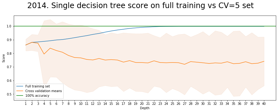
The hyper-parameters of decision trees, random forests and boosting algorithms have been selected by running specific functions plotting indicators from several configurations.
Run cross-validation predictions and compute accuracy
- Here we execute the whole process of folds definition, pre-process, predictions and accuracy computation per each fold and then cross-validate.
- A detailed report is plotted, which helps us understand better the results and the issues
- At the end of the report, we see a plot of how each model performs through the years. Here one example:
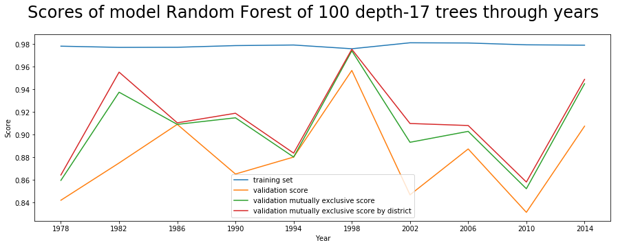
Show models scores
We notice how the single best performing model is random forest, with depth=17 and 100 iterations.
The mean score over the validation folds improved by doing the mutually exclusive selection. This score is still relative to the single candidates.
Then we extract only the predicted winners in each district and we compare them with the party of real winners. That is the validation set mutually exclusive by district.
That last score type is the one we aim to optimize, as our purpose is to predict the winning party in each district.
Feature importance
As random forest is our best model, we select features using the var_sel_RF_2 function, which is a slight variation of the var_sel_RF function from the EDA phase. The main difference is that we don’t need to split the dataset inside the function but we provide the datasets directly as inputs.
Here we run feature importance for each fold from Midterm_recent_years and then show their averages:
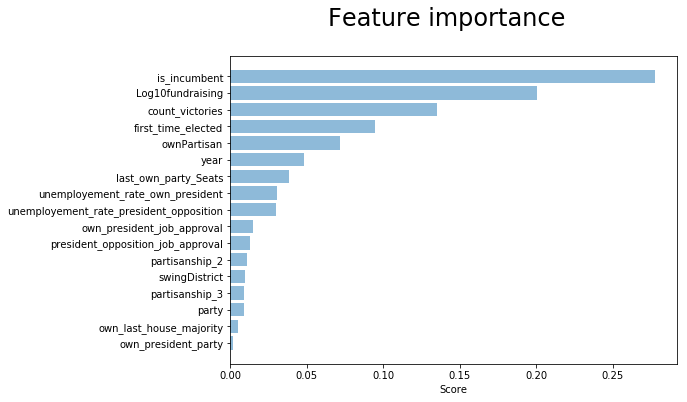
Some of the top features are most probably collinear, like is_incumbent, first_time_elected and count_victories. This influences the behavior and overfit our model.
We could notice how, however, by removing some of the collinear features, even though we might get a more balanced (lower variance) model, we also get lower cross-validation scores.
Stacking
To do stacking, we store the predictions of each model from a list of models into a dataframe, one column per model predictions and one for their probability.
The predictForStack function generates those predictions for each year in a list of years and then appends them together.
We predict results for a list of years (excluding 2018), using the remaining years (still excluding 2018) data as training.
Then we use this data to fit the stacking linear model.
First we generate the predictions for all available models, then we select which models to use to train our stacking model.
The selection is done by looking at the coefficients of the model, taking only the biggest ones.
In our case we get a training accuracy of the stacking model equal to 91.16%.
The stacking model coefficients are: [1.96941015 2.9756576 ].
Then we generate the predictions for 2018 data using all models and stack them according to the selection previously used for model fit.
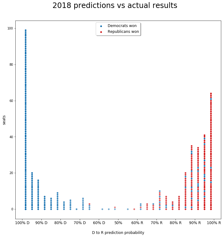
We have obtained our final predictions: the accuracy of our predictions for 2018 midterm elections is 89.89%.
Looking at the sum of predictions:
| Predictions | Actual results | Before elections | |
|---|---|---|---|
| N. Democrat districts | 190 | 230 | 194 |
| N. Republican districts | 245 | 205 | 241 |
Here we see each single district prediction, stacked according to its prediction probability from left (100% probability Democrat), to right (100% probability Republican). The blue or red color gives the actual result of the elections. We can then have a direct idea of the amount and characteristics of the mispredictions.
Hyper-parameters tuning
In order to evaluate the parameters to use for decision trees, random forest and boosting we have performed several cross-validations and plotted the results. Here one example with decision trees depth: